Numeric Integration with techBASIC

Numeric integration, also called quadrature, is a powerful technique for finding the value of the definite integral of a function without having to actually integrate it. It has applications that range from checking your calculus homework to solving real-world problems that are impossible or very difficult to solve analytically.

This article takes a look at how to use numeric integration in techBASIC. We’ll start with a canned program you can use to evaluate practically any integral, and then look at how to quickly modify it for your particular problem. That may be all you are interested in, but if you continue, you’ll dig into the integration program to find out how to customize it, and learn about the different methods techBASIC offers to do numeric integration, which will help you pick the right method for the job.

A Short Program for Numeric Integration in techBASIC

It’s actually not hard to find the integral of a function in techBASIC. This program will do the job

PRINT Math.trap(FUNCTION f, 0, 2)

FUNCTION f (x AS DOUBLE) AS DOUBLE

f = x*x*x*x*LOG(x + SQR(x*x + 1))

END FUNCTION

evaluating

You can easily change the limits of integration in the first line, or change the function that is integrated by changing the next-to-last line. If you are new enough to BASIC that yo don’t see how the equation converts to the function, you might start with the article on using techBASIC as a graphing calculator—it gives more detailed examples showing how to create and change functions in BASIC.

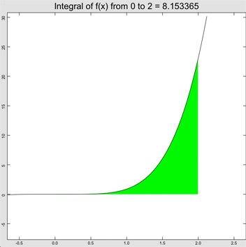
While that works, it just scratches the surface of what we should expect from a good technical computing package. Here’s a program that will perform the numeric integration, but it also plots the result, shows the area under the curve, and displays the answer in the title of the plot. This is a great way to understand the answer and look for potential problems, like discontinuous functions.

While you can type the program in manually, you can also copy the program from the article and paste it into an empty techBASIC program, or download the completed program from the end of the article and move it to techBASIC using iTunes. If you’re not familiar with how to do that, see the Quick Start guide on the techBASIC documentation page.

! Set up the limits of integration and find the integral.

x0 = 0

x1 = 2

ans = Math.trap(FUNCTION f, x0, x1)

! Create a plot to show the function and result.

DIM p AS Plot

p = Graphics.newPlot

! Draw the area under the curve.

DIM intfx AS PlotFunction

intfx = p.newFunction(FUNCTION f)

intfx.setDomain(x0, x1)

intfx.setFillColor(0, 1, 0)

intfx.setColor(0, 1, 0)

! Draw the function that was integrated.

DIM fx AS PlotFunction

fx = p.newFunction(FUNCTION f)

! Start by showing the area integrated in the middle 60% of the

! plot, with some buffer around the edges to see the part of the

! function that was not integrated.

minY = f(x0)

maxY = f(x1)

FOR x = x0 TO x1 STEP (x1 - x0)/100

y = f(x)

IF y < minY THEN minY = y

IF y > maxY THEN maxY = y

yRange = maxY - minY

minY = minY - yRange/3

maxY = minY + yRange*5/3

minX = x0

IF x1 < minX THEN minX = x1

minX = minX - ABS(x1 - x0)/3

maxX = minX + ABS(x1 - x0)*5/3

p.setView(minX, minY, maxX, maxY, 0)

! Use the plot title to show the limits of integration and the result.

p.setTitle("Integral of f(x) from " & STR(x0) & " to " & STR(x1) & " = " & STR(ans))

p.setTitleFont("Sans-Serif", 25, 0)

! Display the plot.

System.showGraphics

! This is the function to integrate.

FUNCTION f (x AS DOUBLE) AS DOUBLE

f = x*x*x*x*LOG(x + SQR(x*x + 1))

END FUNCTION

Using Our Program and Dealing With Discontinuities

So how can we put this program to use? Let’s start with a calculus problem. I found this one on a web site that has practice problems.

Evaluate the definite integral

where

Change the function to

FUNCTION f (x AS DOUBLE) AS DOUBLE

IF x <= 1 THEN

f = x*x + 2*x + 3

ELSE

f = SQR(4*x)

END IF

END FUNCTION

Now when we run our program, we get… an error! techBASIC says, “Runtime error: Desired accuracy was not achieved in the allowed number of steps.”

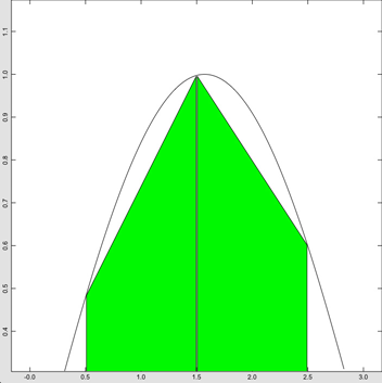
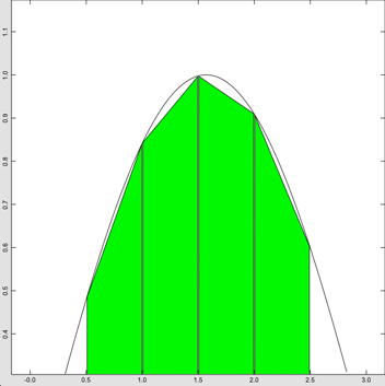
It’s important to understand a little about how numeric integration works to understand why this happened. The trapezoid rule, which is what we’re using, starts off by evaluating the function at the end points and middle. The first approximation to the integral is formed by finding the area under the two trapezoids. Next, each trapezoid is divided in half, and a new approximation is made from the four trapezoids. The two values are compared, and if they are closer than a specified allowed error, the integral returns with the answer. If not, the process is repeated, splitting the polygons in half again and again.

Friday, May 18, 2012

This can take a really long time if there is a sharp jump in the function somewhere, and for some functions, the error may never get small enough. To prevent that, there is a limit on the number of times the trapezoids are divided in half before the routine gives up.

There are three ways we can deal with this problem. The first is to change the allowed error. Looking at the online help system, we see that Math.trap actually has five parameters, not just the three that we used. The fourth parameter is the allowed error, which defaults to 10-6, giving about 5 digits of precision. Drop that to three digits of precision by changing the line

ans = Math.trap(FUNCTION f, x0, x1)

ans = Math.trap(FUNCTION f, x0, x1, 1e-4)

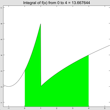
and try again. Now we get an answer, and we can also see the problem. There is a sharp discontinuity at x=1.

Well, this shouldn’t really stop us from evaluating the integral, it will just cause it to take a lot longer. Change the error back to 1e-6 and try increasing the number of allowed steps from the default of 16 to 25.

ans = Math.trap(FUNCTION f, x0, x1, 1e-6, 25)

The program takes a lot longer to run, but does give an answer to five significant digits.

So does this do our calculus homework for us? Not really. We’ll still need to show our work, but it does help make sure we got the right answer. When we solve the integral analytically, we get 41/3 for an answer. This agrees nicely with 13.6666, giving us confidence that the analytic solution is correct.

Problems With Regular Functions

Let’s try another one. This time we’ll integrate

by changing the function to

FUNCTION f (x AS DOUBLE) AS DOUBLE

f = ABS(SIN(x))

END FUNCTION

and at the top of the program, the second limit of integration from

x1 = 4

x1 = 4*Math.PI

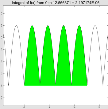
Run the program. OK that’s not good. Clearly the answer is not zero, but that’s what we get to five significant digits. Remember how trapezoidal integration works, though? Taking the first, last, and middle point, f(x) is zero in each case. Divide the polygons in half and try again, and we still have points where f(x) is zero. That’s why a program like the one we’re using is nice. We can see from inspection that the answer is nonsense, and a little knowledge of how trapezoidal integration works tells us why. If it had only evaluated one more step, the integration routine would have found some non-zero points and continued on, giving a good answer.

To solve this problem, we’ll drop back to a less sophisticated version of the trapezoid rule that doesn’t look for the difference between successive evaluations to decide when to stop, it simply evaluates the integral by dividing the trapezoids in half a specific number of times. Math.trapf does this.

Change the line that evaluates the integral from

ans = Math.trap(FUNCTION f, x0, x1)

ans = Math.trapF(FUNCTION f, x0, x1)

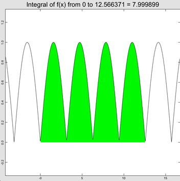
Run the program again, and the answer is 7.999599, much closer to the correct value of 8. Of course, we may want to change the number of iterations manually to get an idea of the accuracy. Checking the help files, we see that Math.trapf defaults to 10 steps. Change that to 11 by modifying the line that does the integration to read

ans = Math.trapF(FUNCTION f, x0, x1, 11)

and the answer changes to 7.999899, showing that the answer is good to four digits.

Polynomial Integration Methods

If you’ve looked at numeric integration before, you might wonder why we’ve used trapezoidal integration up to this point. The famous Simpson’s Rule gets results a lot quicker by fitting a curve to three successive points rather than using a straight line, like the trapezoid rule. The reason is that the trapezoid rule is about as foolproof as a numeric integration method can be. Other than using a function that isn’t defined at all at some point in the area we want to integrate, the only two problems it faces are the two we’ve already looked at, and a simple plot of the function helps avoid nonsense answers or helps show us why a function might not converge to the accuracy we want quickly enough. When polynomial fits are applied, there are new problems that we have to deal with. Discontinuities in the first derivative cause the same sorts of problem in Simpson’s Rule that we already saw with the trapezoid rule when the function was discontinuous. The function has to be “sufficiently smooth” to use the polynomial methods of integration. For Simpson’s Rule, that generally means a continuous first derivative. For Romberg integration, which can apply even higher orders of polynomials, the second derivative should be continuous for polynomials with an order of 3, the third derivative should be continuous for polynomials with an order of 4, and so on.

But if the function is smooth enough, Romberg integration can be blazingly fast.

Let’s take a look at the first function we evaluated. Change the function being integrated back to

FUNCTION f (x AS DOUBLE) AS DOUBLE

f = x*x*x*x*LOG(x + SQR(x*x + 1))

END FUNCTION

and the second limit of integration to

x1 = 4

then run the program. The answer of 389.961823 pops up pretty fast. Now change the line that evaluates the integral to

ans = Math.romb(FUNCTION f, x0, x1)

and try again. This time the answer is 389.961761, but the answer is still there pretty quickly.

Now let’s try something different. Rather than evaluating the function one time, let’s evaluate it 250 times and record the time it takes to do so. Replace the line that integrates the function with

time& = System.ticks

FOR i = 1 TO 250

ans = Math.romb(FUNCTION f, x0, x1)

PRINT "Elapsed time = "; System.ticks - time&

The program still seems to run pretty quickly, but there is a noticeable pause. Now change from Romberg integration to the trapezoid rule by changing romb to trap, and try again. The difference is dramatic—my times showed that Romberg integration was 16 times faster than trapezoid integration!

Some people might be tempted to use Romberg integration as the default method of integration, but remember that the function has to be sufficiently smooth. That’s why I recommend using the trapezoid rule when an integral only has to be evaluated once, or at most a few times. If you are writing a program that will be evaluating an integral many times, or evaluating the integral in a time-sensitive part of the program, it’s worth using Romberg integration—but only after making sure the function is smooth enough.

Back at the start of this section, we talked about Simpson’s Rule. So where is it? It turns out that Simpson’s Rule is a subset of Romberg integration. Taking a look at the help file, you see that Romberg integration has three optional parameters. The first two are the desired accuracy and maximum number of steps, just like for the trapezoid rule. The last gives the polynomial order, which defaults to 5. Setting the order to 2 tells Romberg integration to use a second order polynomial, which is what Simpson’s Rule uses.

It’s worth playing with the order when using Romberg integration many times on a specific function. The default order of 5 is a good starting point, but lower orders may give an answer just as fast for some functions, and higher orders may work better for others. Don’t automatically pump the order up, though—eventually, round off errors start to accumulate, and accuracy suffers. You may get the dreaded “Runtime error: Desired accuracy was not achieved in the allowed number of steps.” if you specify an order that is too large.